Modelling Electron Cut-out Factors
by Simon BiggsSupervisors:
- John Kenny
- Konstantin Momot
- Andrew Fielding
Overview
- Background
- Linac collimation
- Scatter effects
- Electron output factor
- Objective
- Method
- Smoothing spline
- Uncertainty
- Give, gap, and slope
- Fit flexibility
- Validation
- Results and Discussion
- Validated fits
- Fits not validated
- Outliers
- Validation
- Model demonstration
- Conclusion
- Improvements and future directions
- Questions
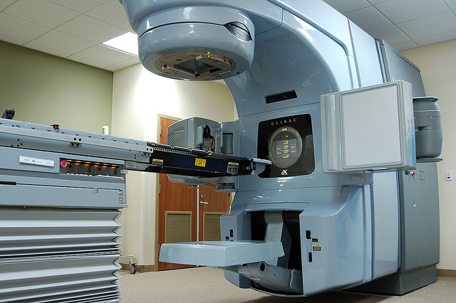
Electron beam collimation
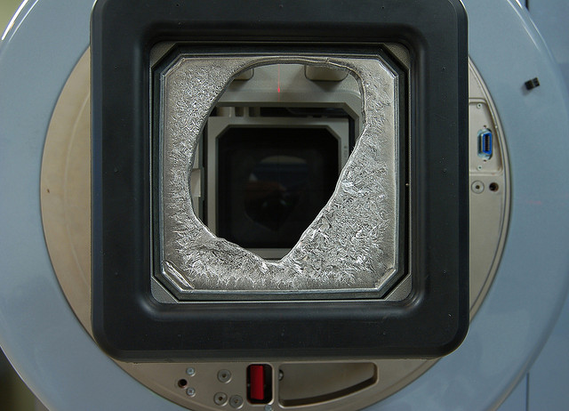
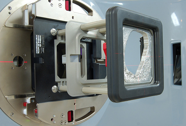
Collimation
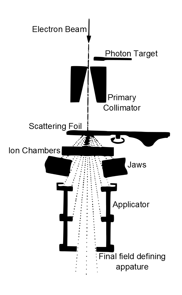
Faiz M Khan and F Khan. The physics of radiation therapy, volume 3. Lippincott Williams & Wilkins Philadelphia, 2003.
Scatter effects
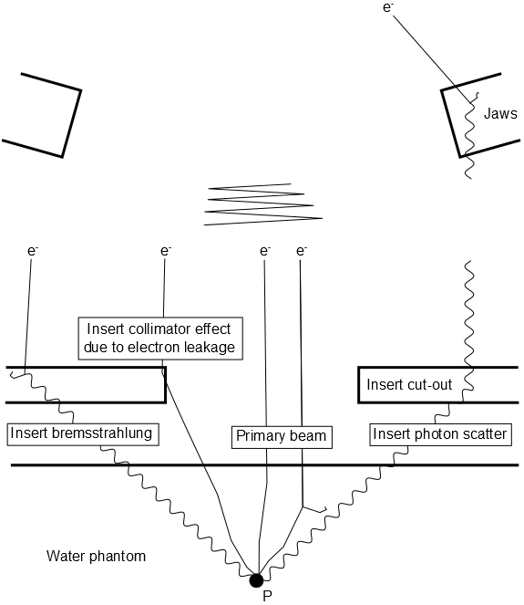
BA Faddegon and JE Villarreal-Barajas. Final aperture superposition technique applied to fast calculation of electron output factors and depth dose curves. Medical physics, 32:3286, 2005.
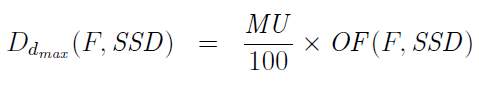
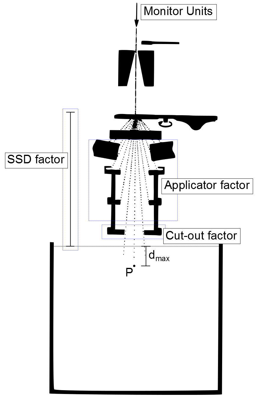
The electron output factor
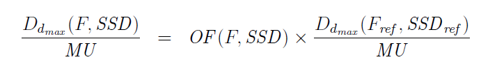
Faiz M Khan, Karen P Doppke, Kenneth R Hogstrom, Gerald J Kutcher, Ravinder Nath, Satish C Prasad, James A Purdy, Martin Rozenfeld, and Barry LWerner. Clinical electronbeam dosimetry: Report of AAPM radiation therapy committee task group no. 25. Medical physics, 18:73, 1991. 2005.

Objective
To predict electron cut-out factors that have been measured in a water tank with a known uncertainty.
Method
Advantages of the method used
- Only needs cut-out factors that have already been measured
- Takes the input of cut-out shape length and width
- Increased accuracy compared to basic interpolation
- Gives the uncertainty in the cut-out prediciton
- Reduces the frequency that factors need to be measured
- Can be used to increase the accuracy of a pencil beam model
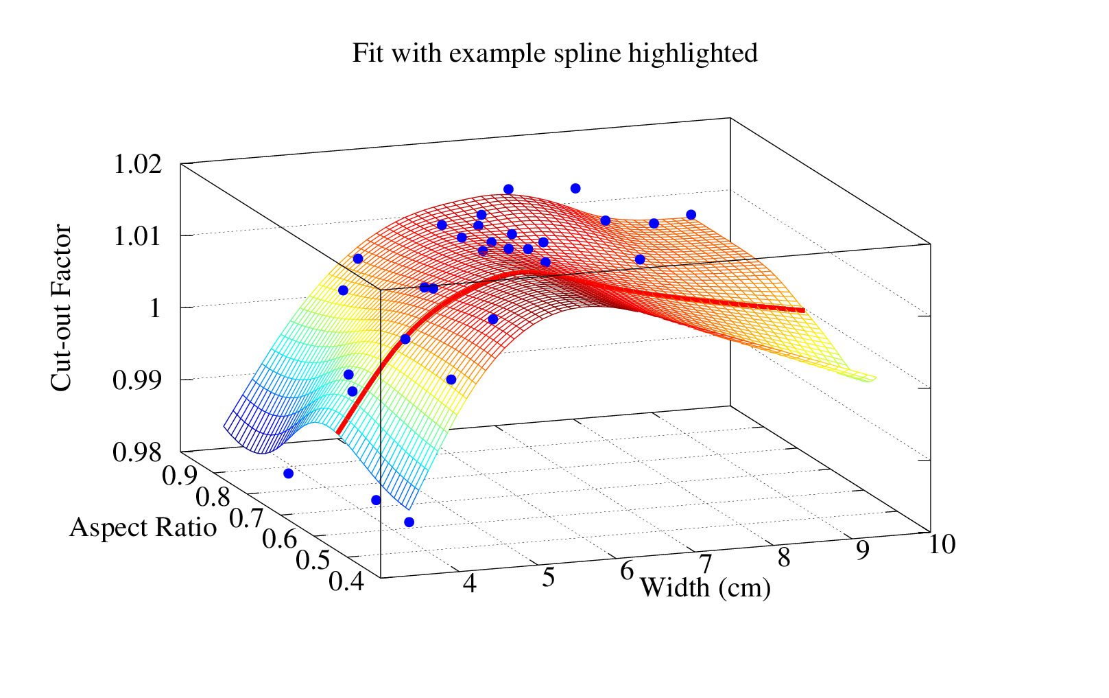
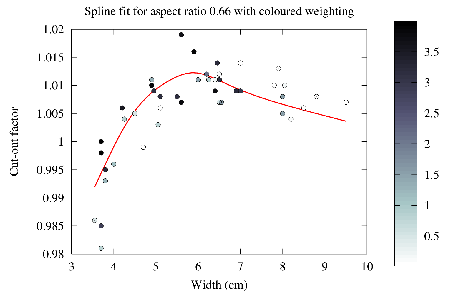
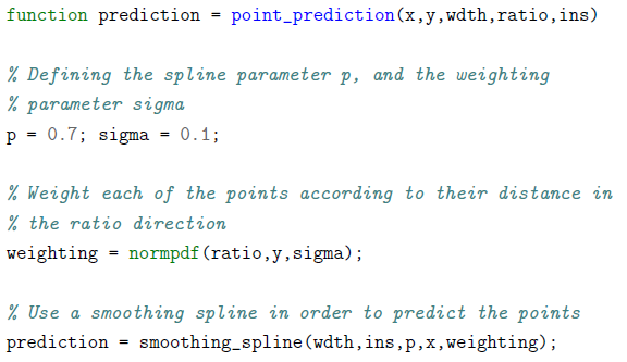
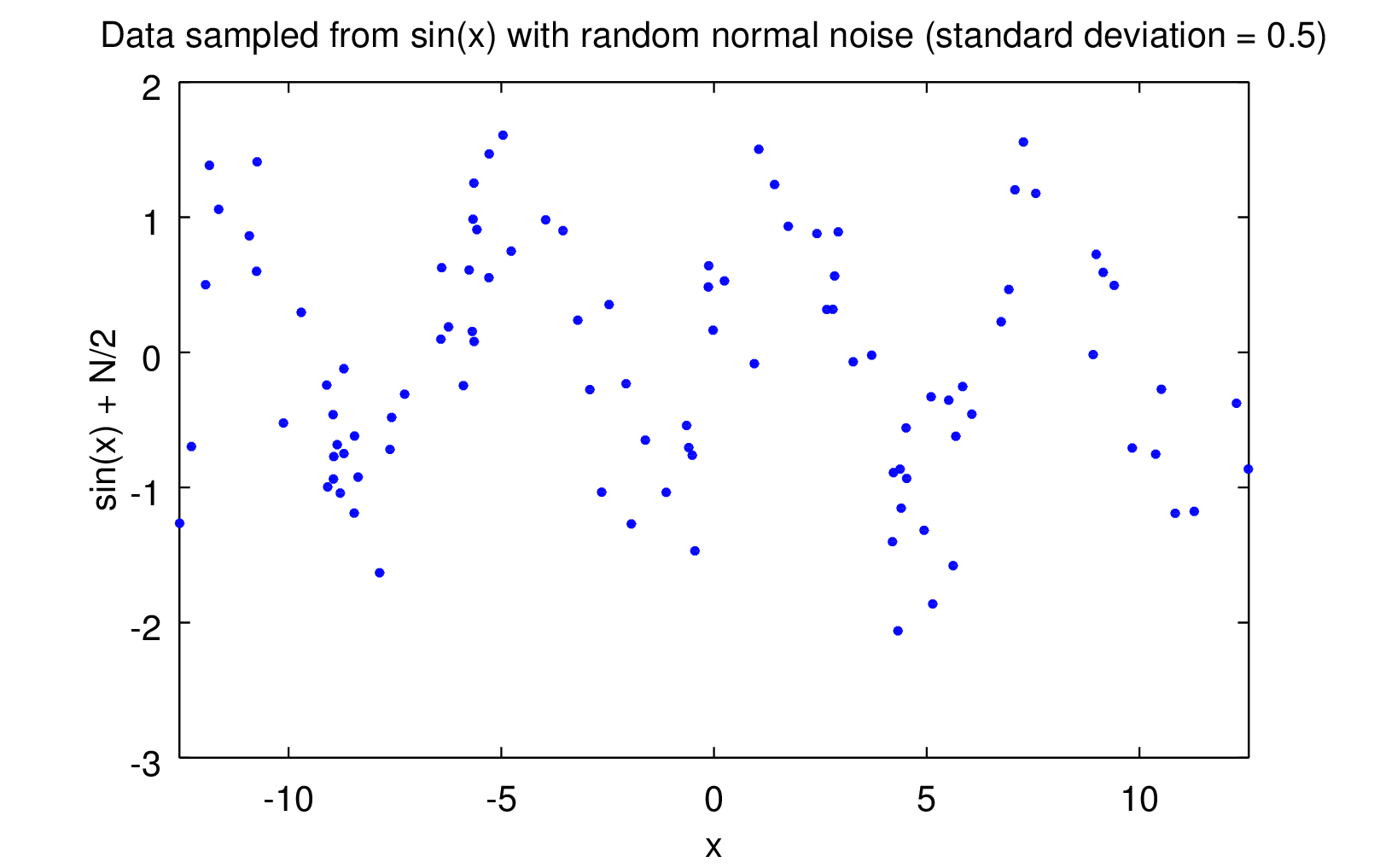
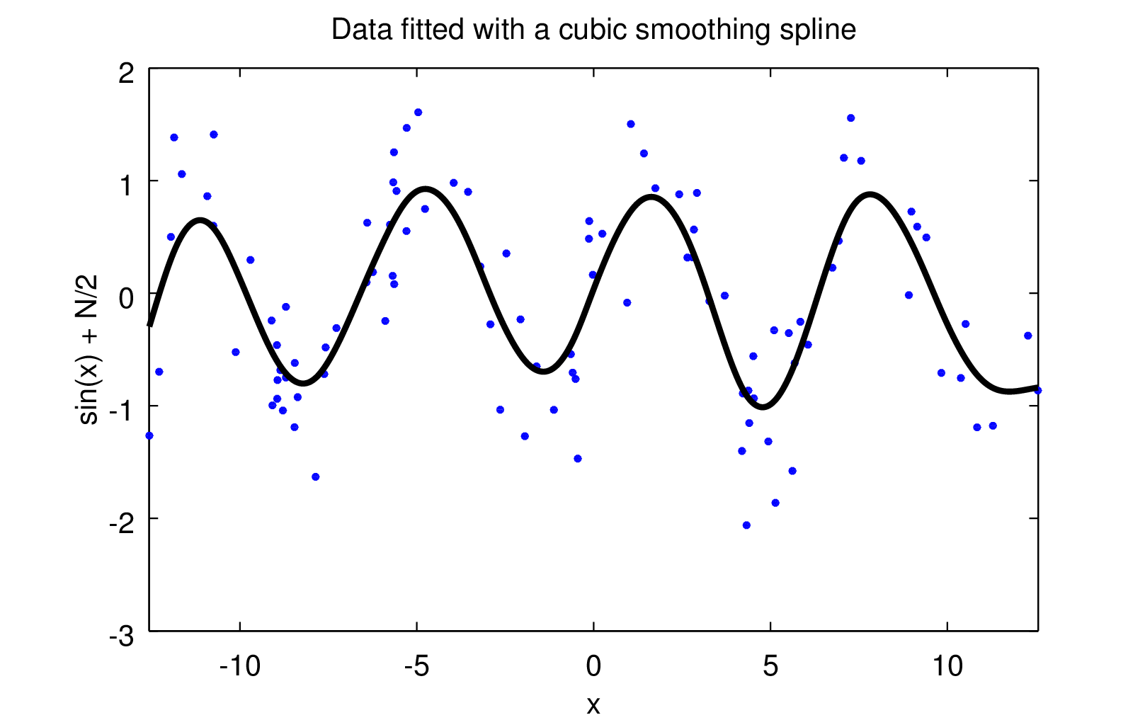
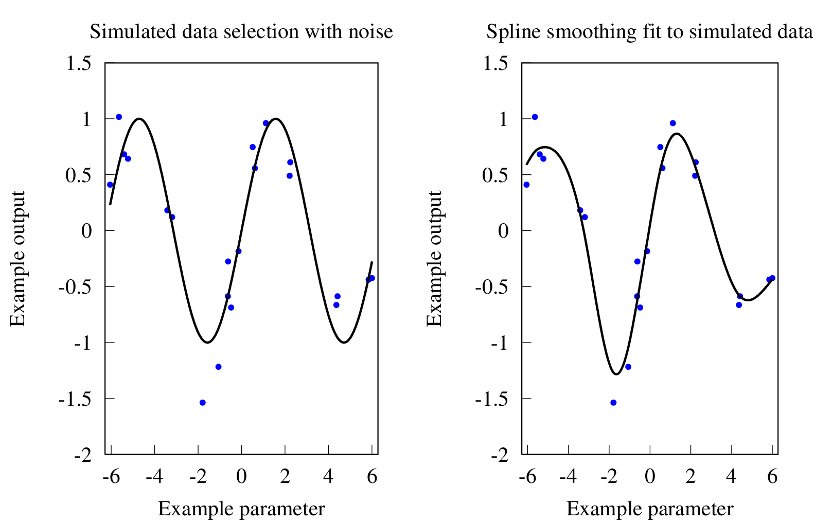
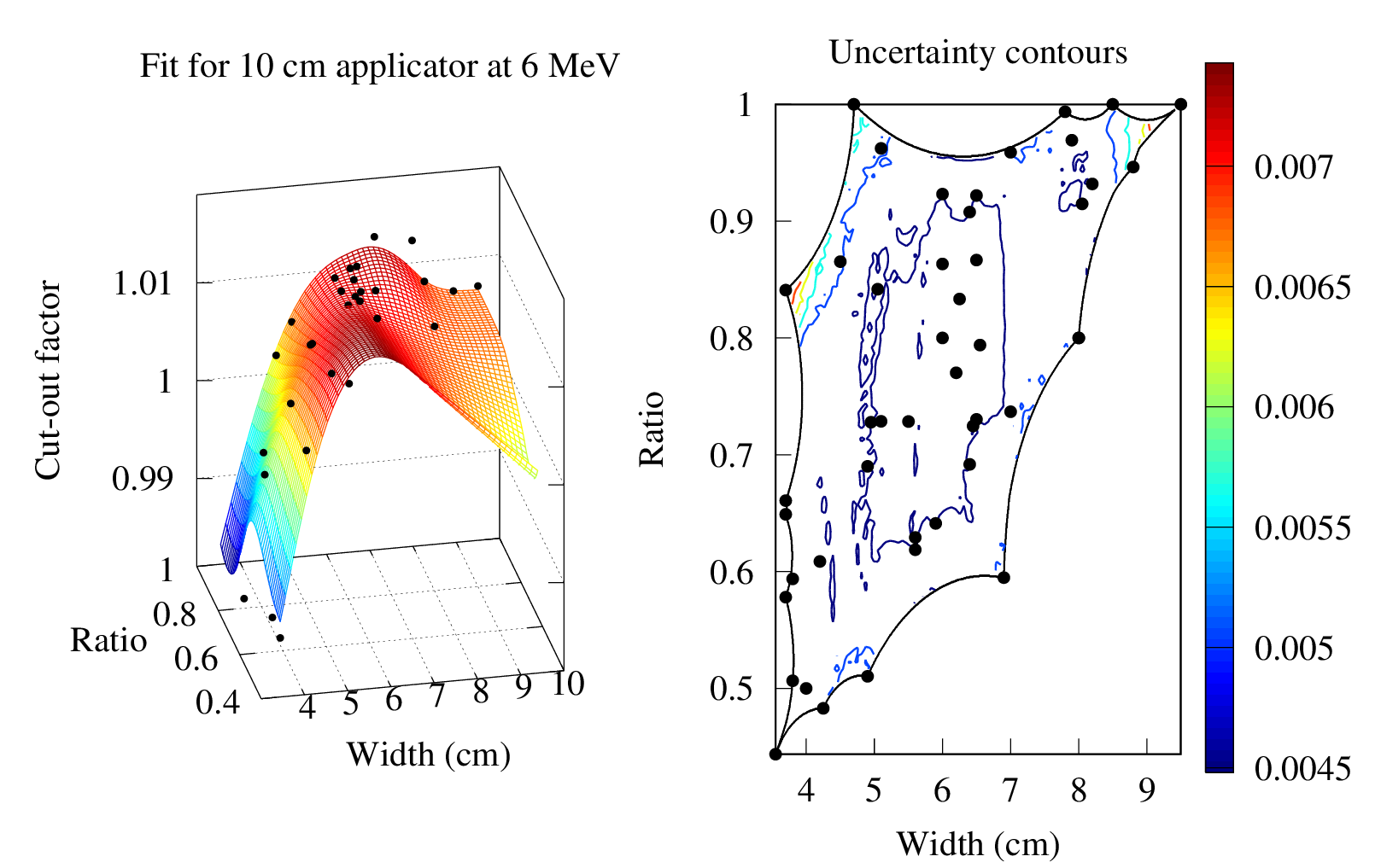
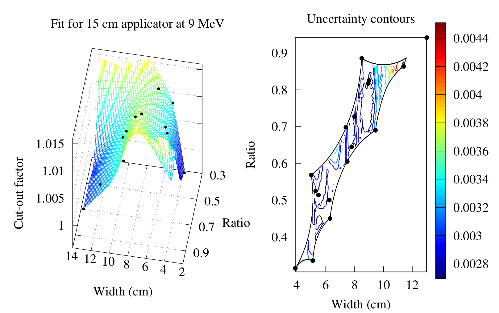
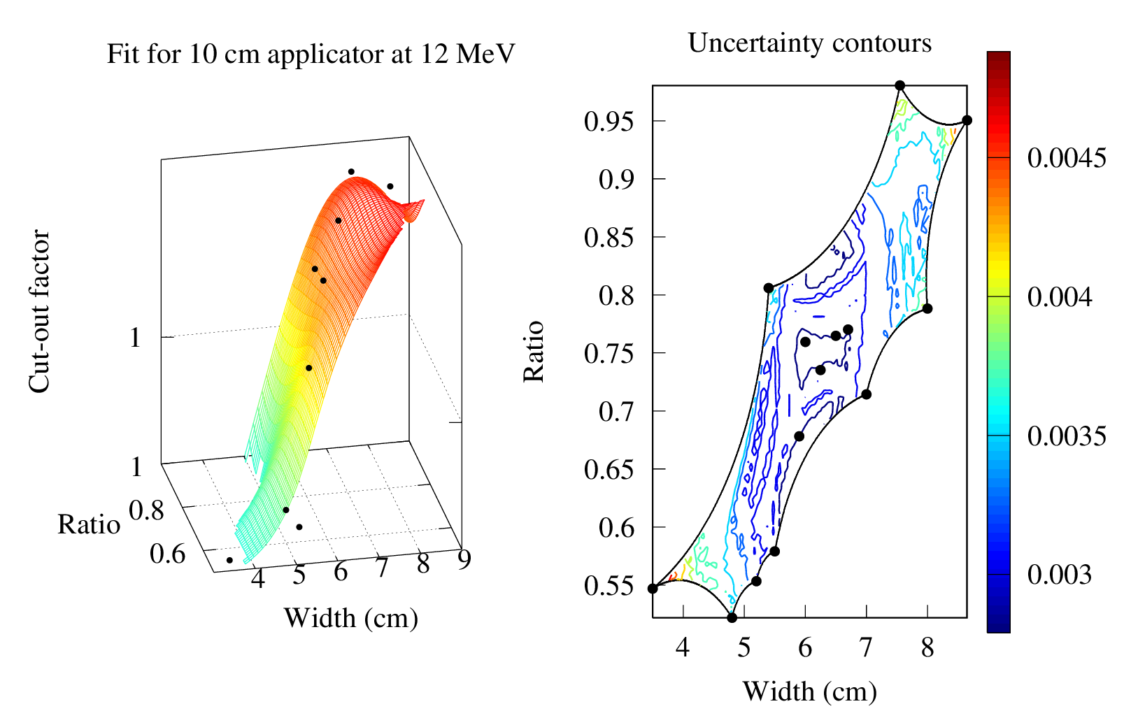
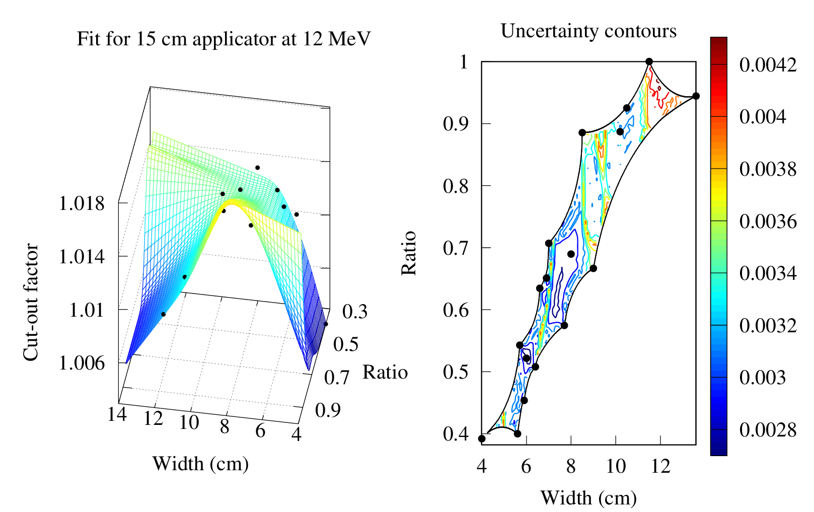
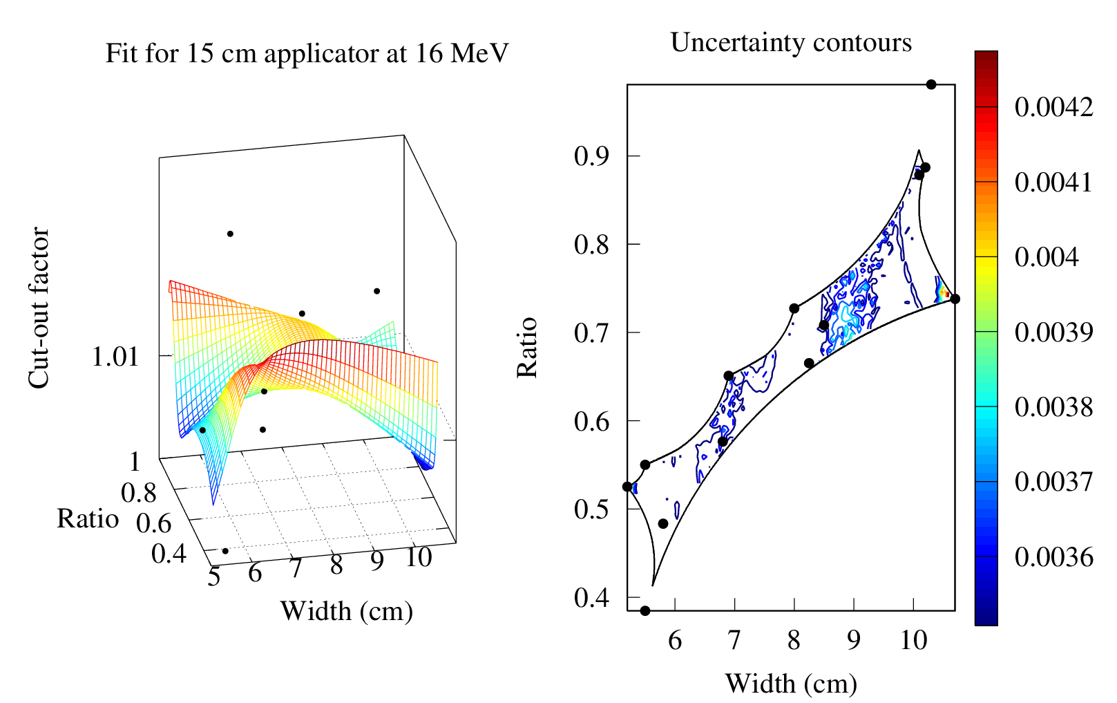
Smoothing Spline
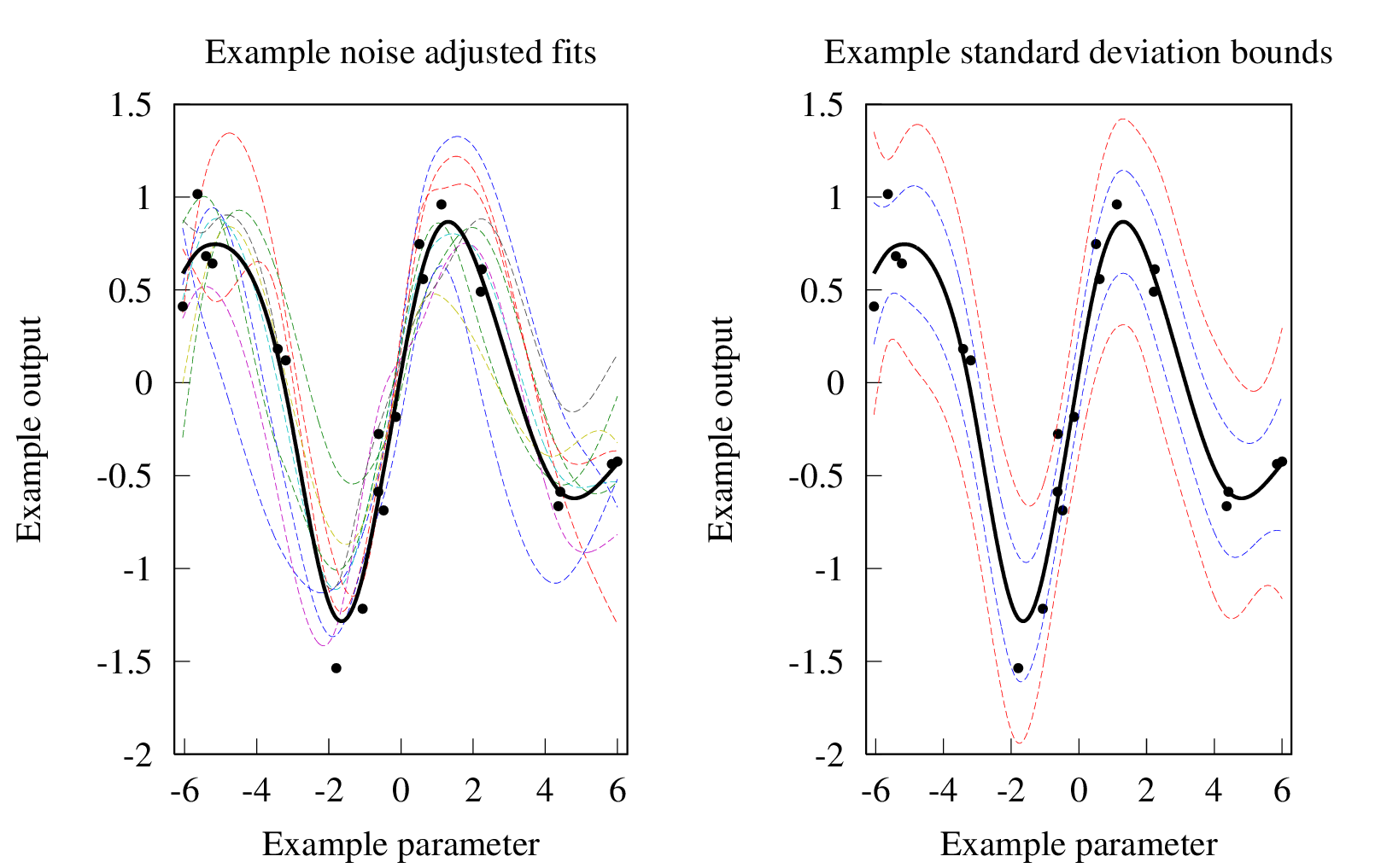
Determining the Uncertainty
- Defined a lower bound uncertainty by:
- Predicting measured points after their removal
- Compared to the region parameters give, gap, and slope
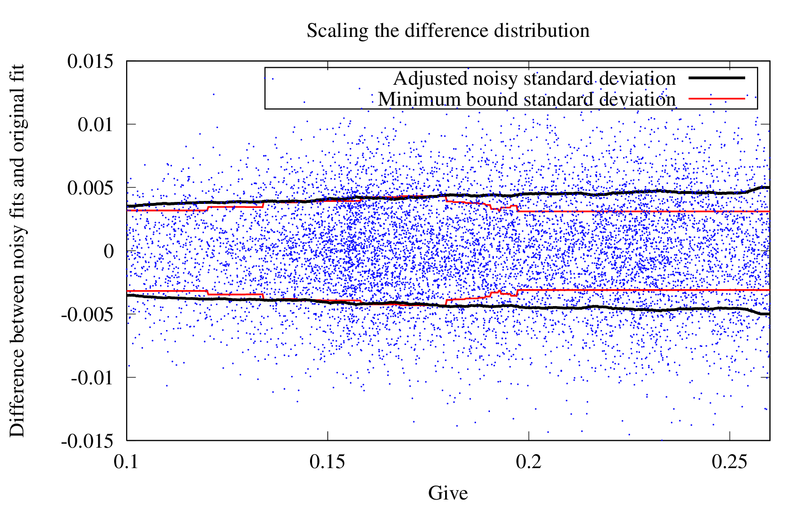
- Fit flexibility calculated by:
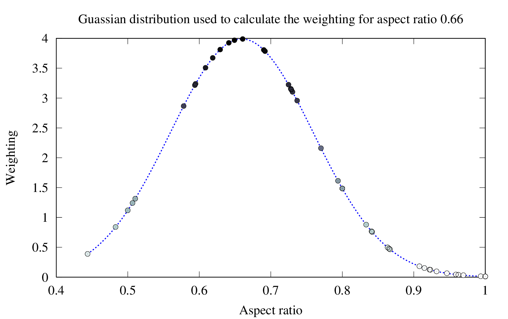
- Added Guassian noise to all measured cut-out factors
- Created fit with new noisy data
- Repeated 10 000 times creating a set of fits
- Took the standard deviation of the set of fits
- Compared to the region parameters give, gap, and slope
- Uncertainty determined by:
- Scaled flexibility to be above the lower bound uncertainty
- Used maximum uncertainty predicted by the parameters
Need for Region Parameters
Three parameters
- Give – to determine outlier influence and number of points in a particular region
- Gap – to determine the boundary definition
- Slope – to weight regions of higher gradient accordingly
Give
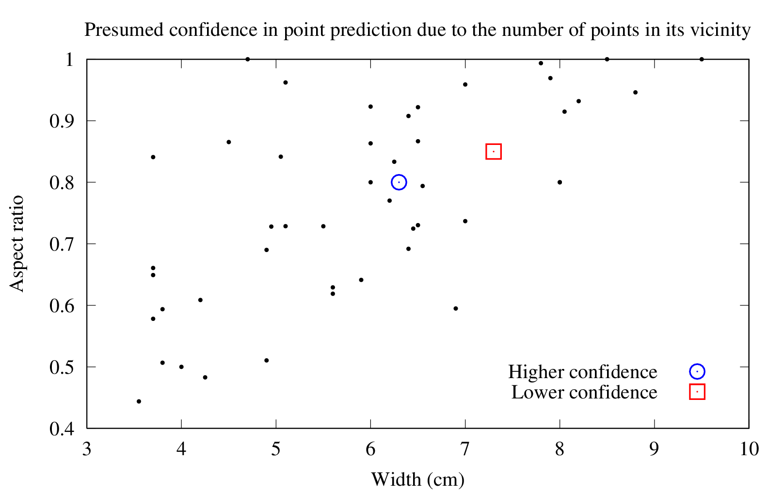
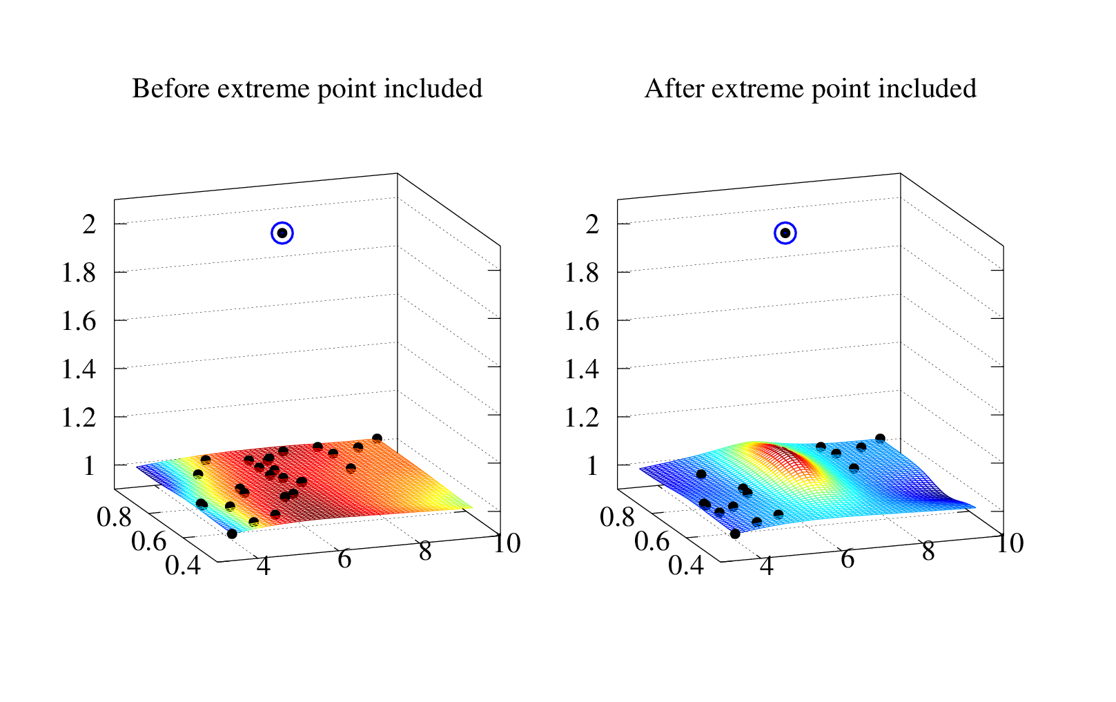
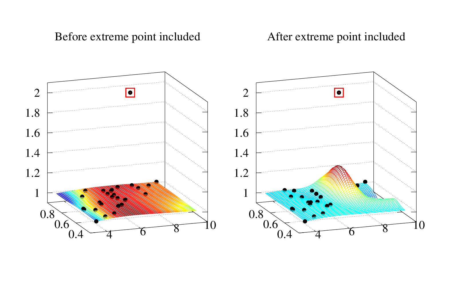
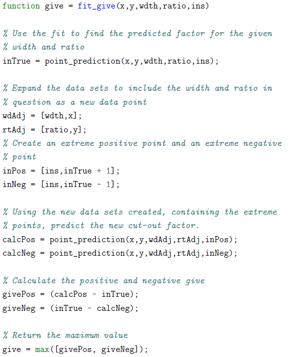
Give calculation
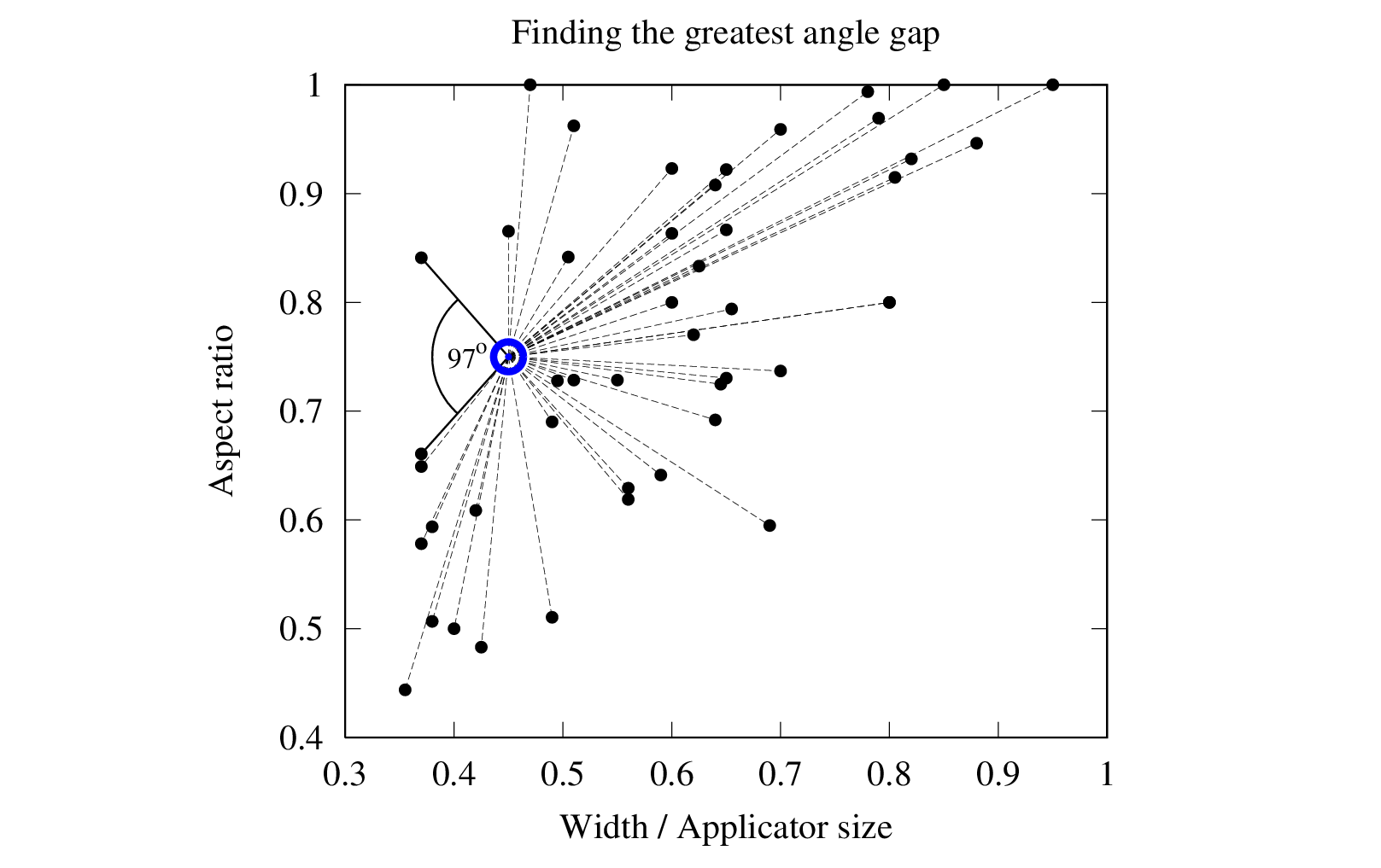
Gap
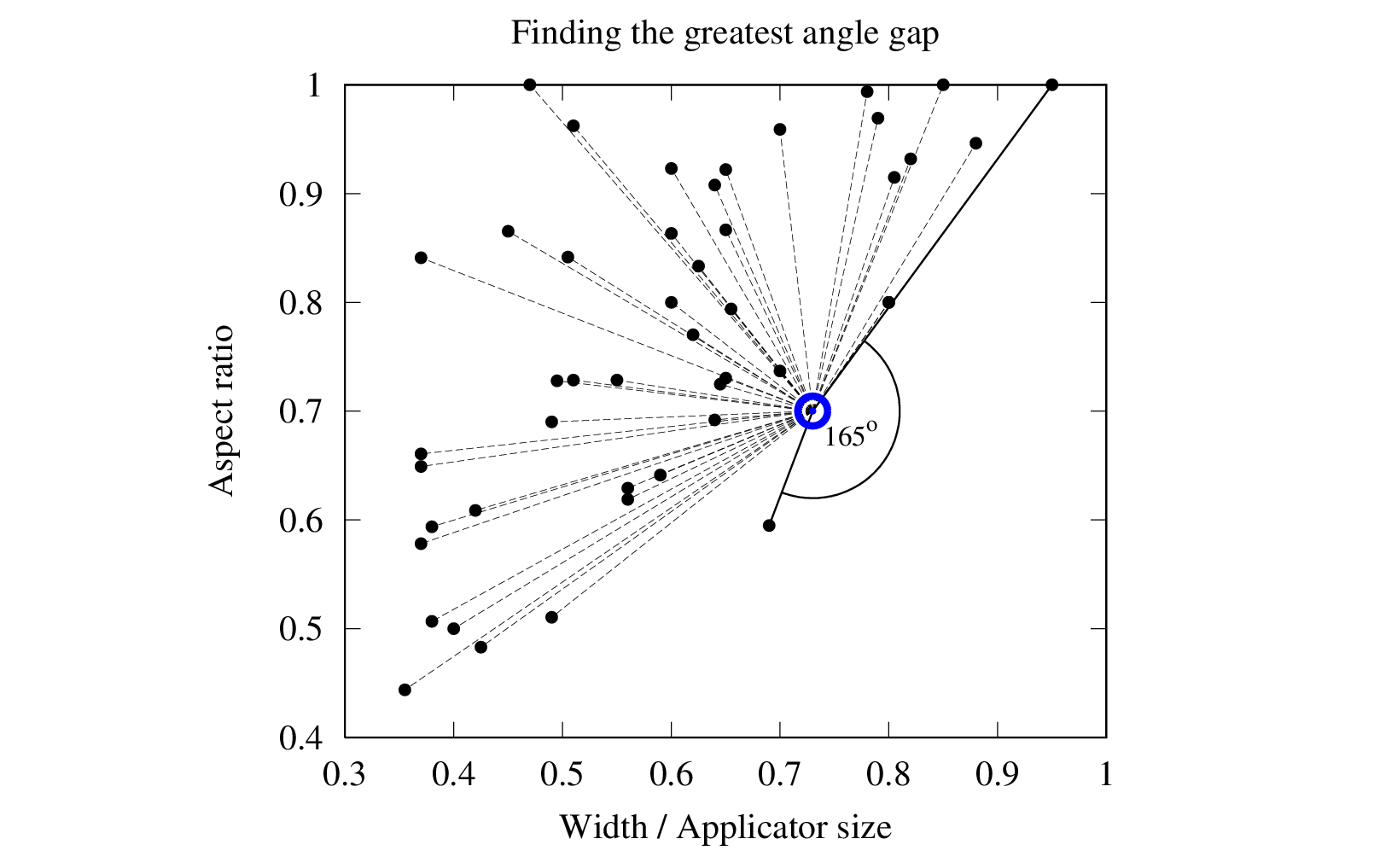
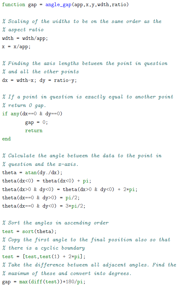
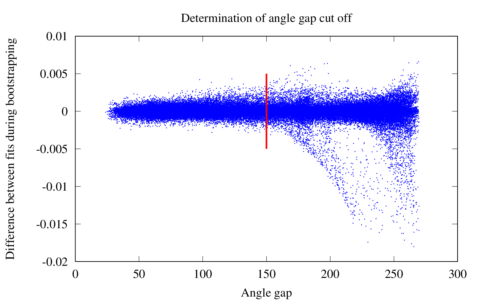
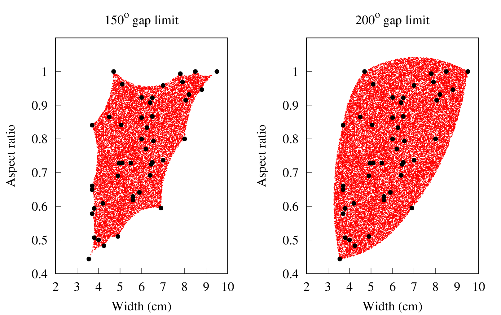
Gap cut-off
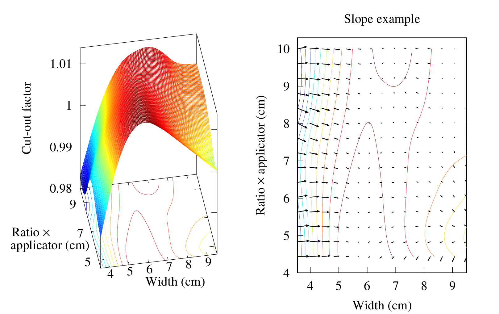
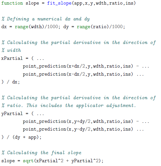
Slope
Fit flexibility
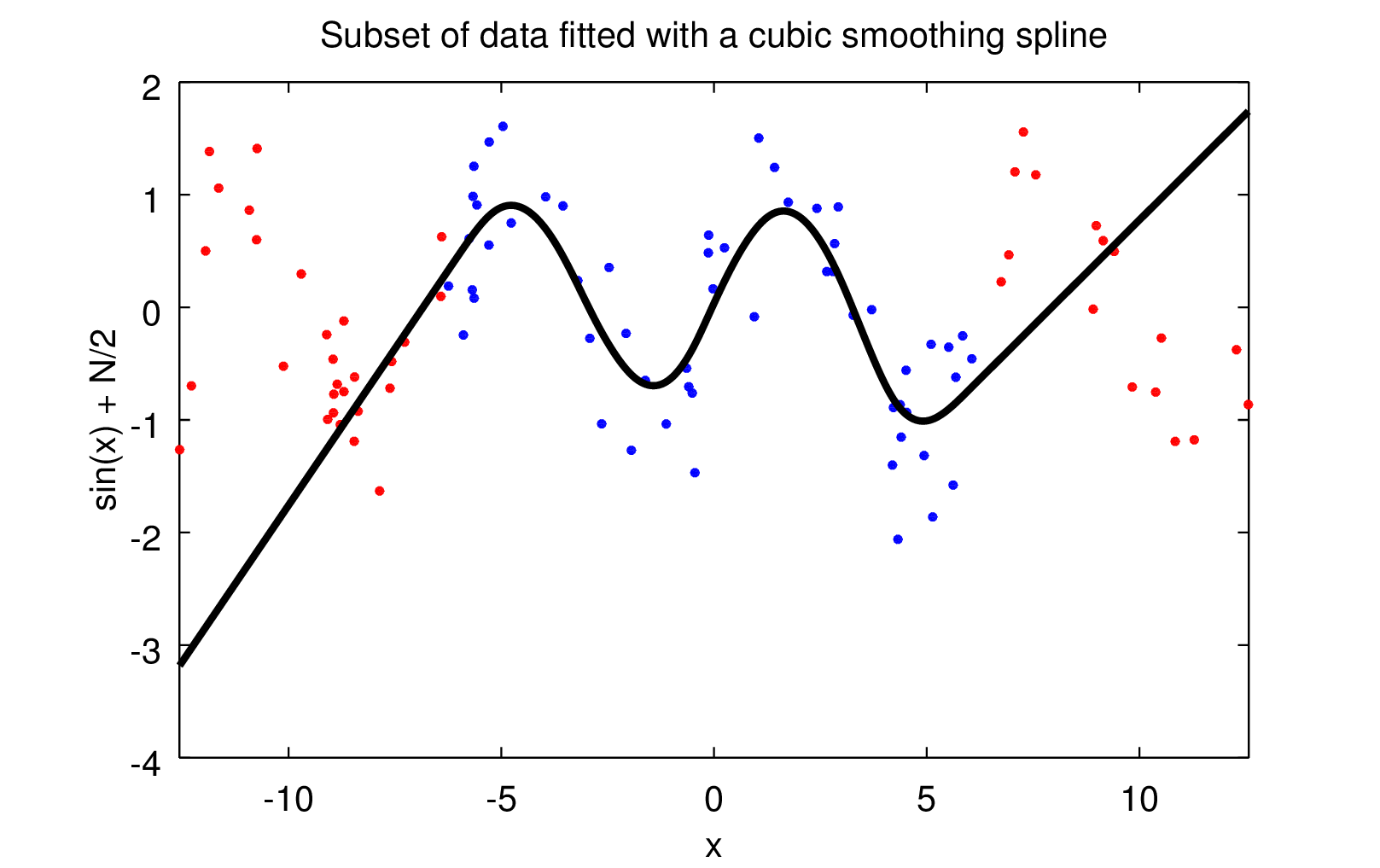
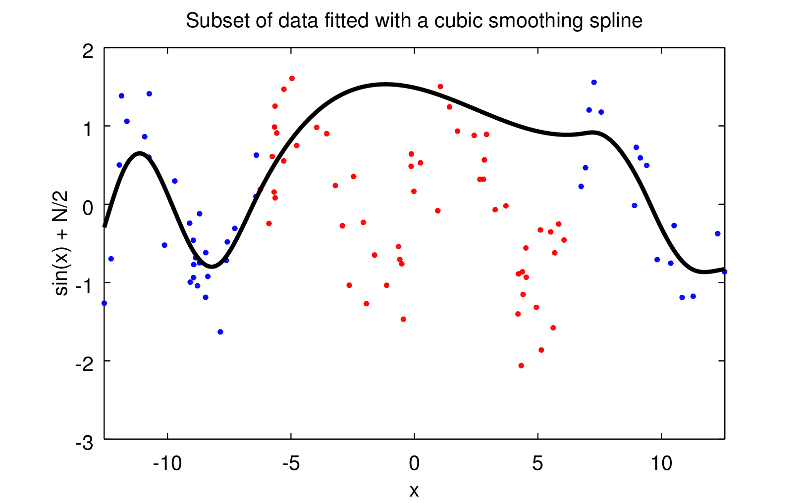
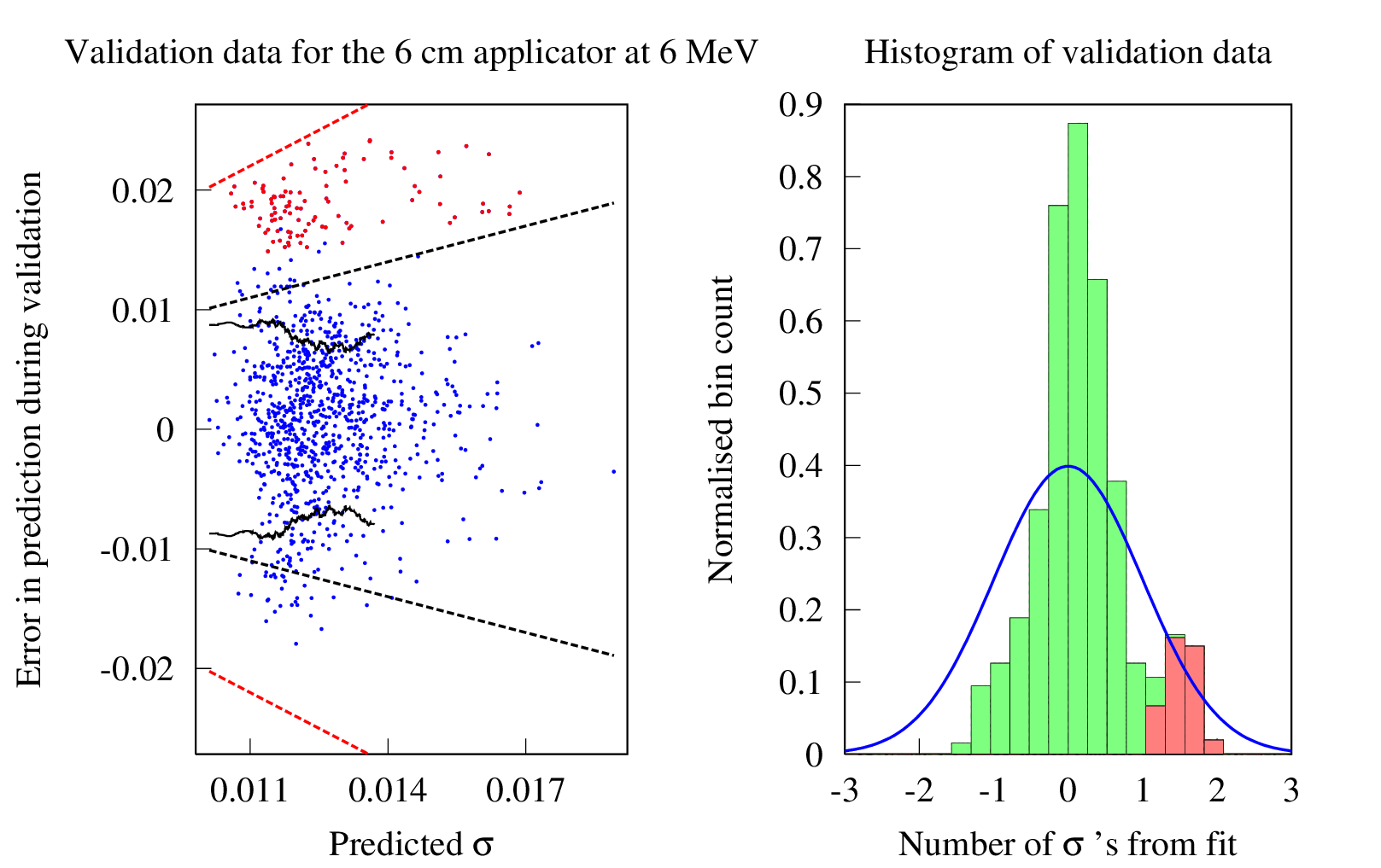
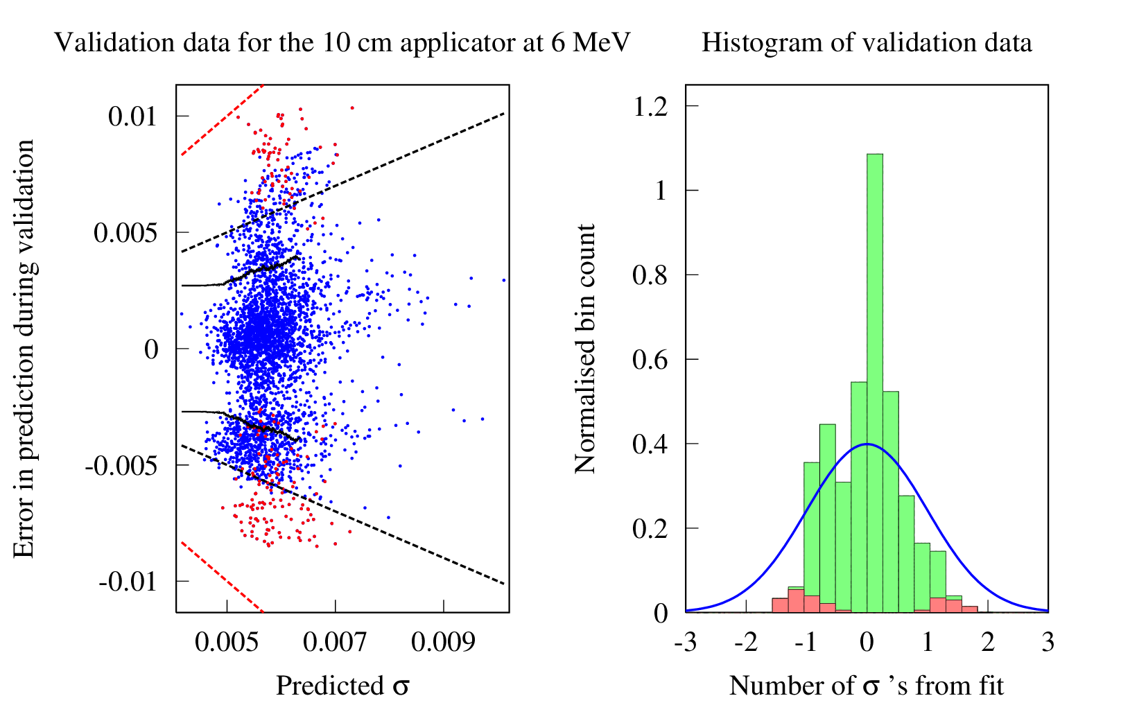
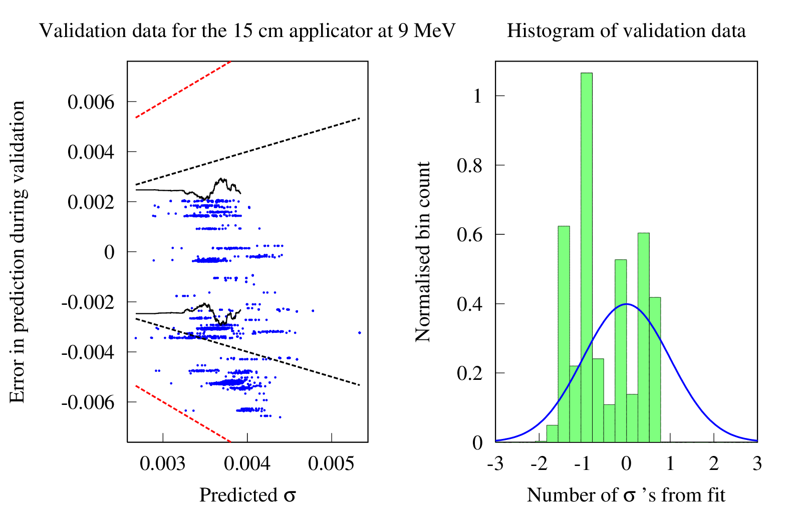
Validation
- Fitting procedure was repeated with a random subset of data points
- This subset fit was used to predict the removed data points
- This was repeated
- The predicted uncertainty was compared to the prediction errors in the removed data points
- A fit was deemed valid should an error greater than 2 SD occur no more than than what would be expected by the Gaussian distribution
Results and Discussion
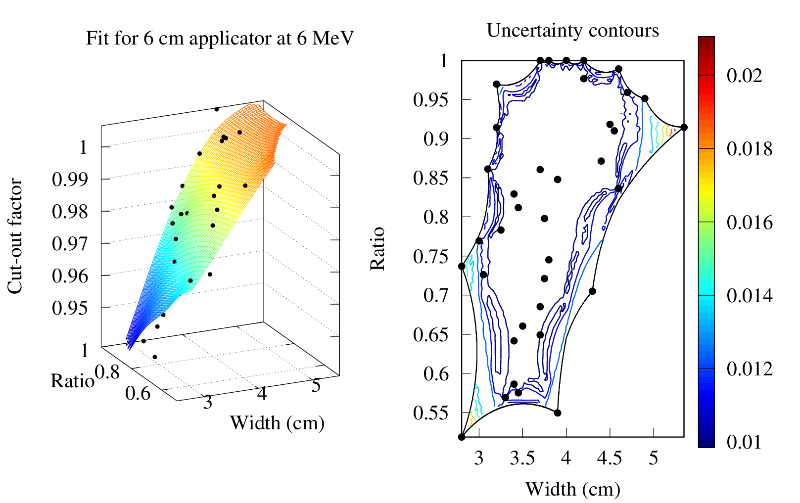
Validated fits
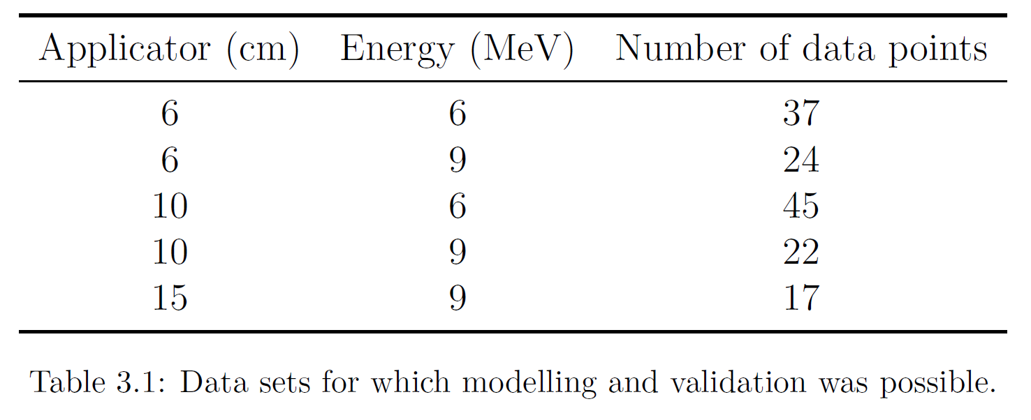
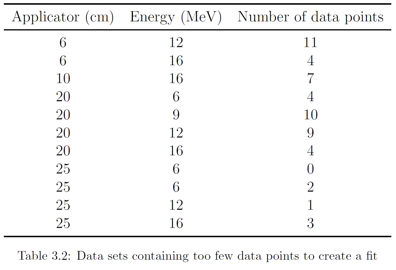
Not enough measured data
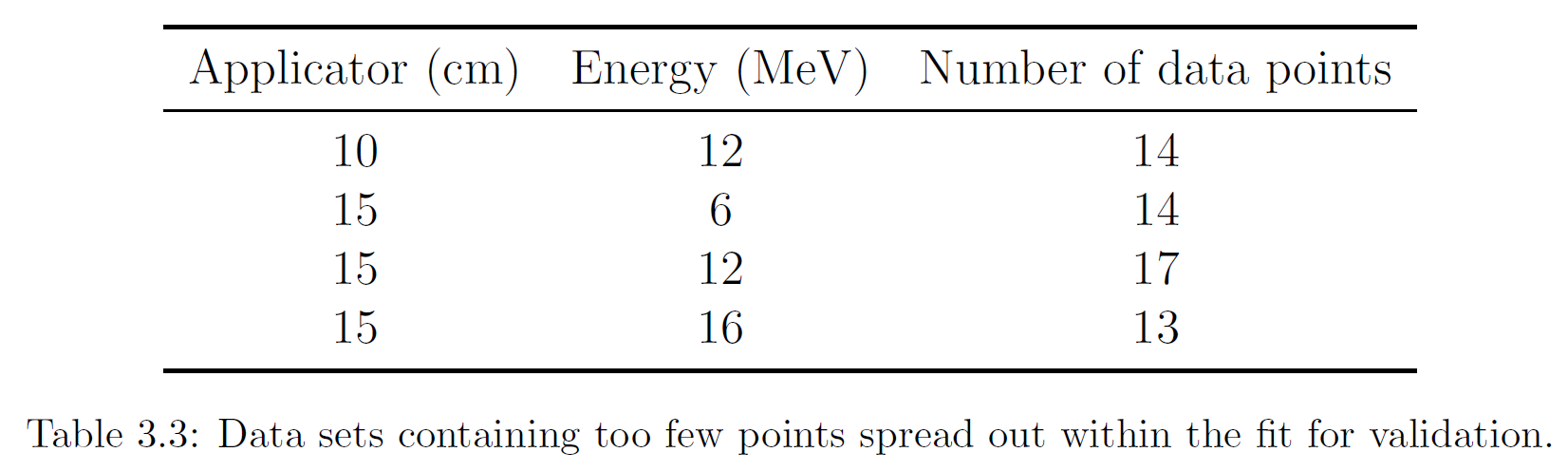
Too few points within boundary
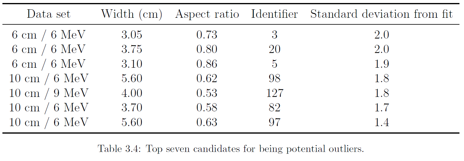
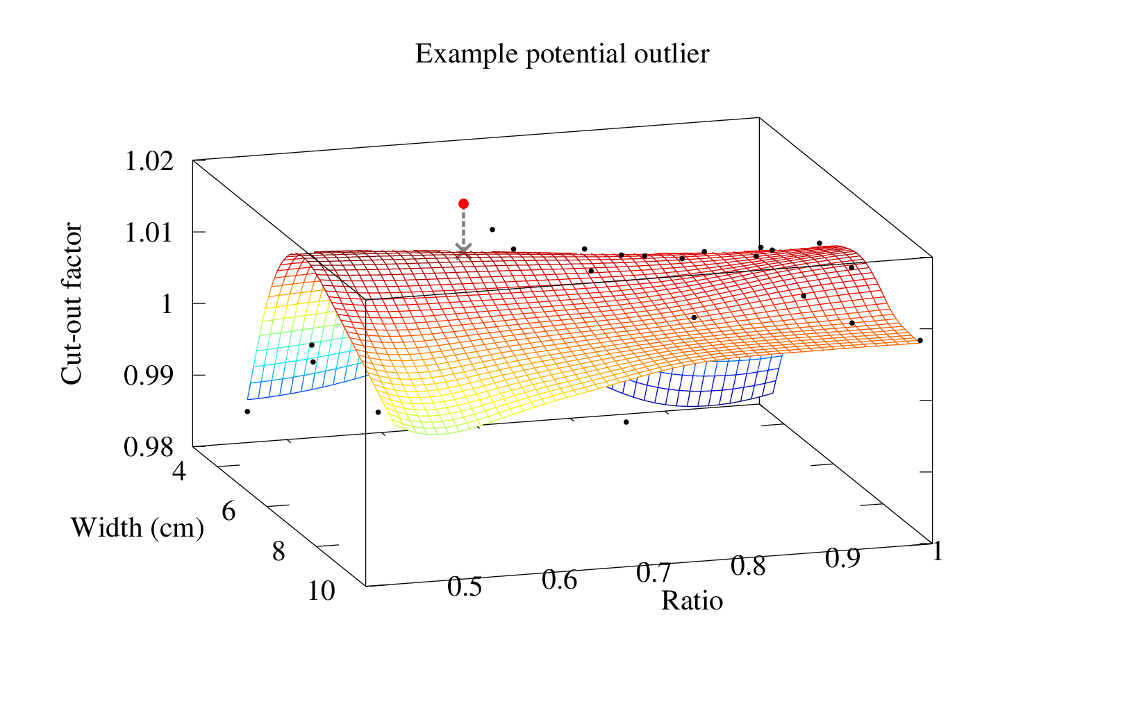
Potential Outliers
Validation
Model Demonstration
Conclusions
Improvements and Future directions
- Effective clinical implementation
- Well defined length and width measurement
- User friendly
- Improved use of slope parameter
- Propegate measurement uncertainty
- Further data collection in sparse regions
- Shape detail
- Area and perimeter
- Model lateral scatter separately
- Sector integration
- Patient geometry
- Adapted pencil beam model
- Use scipy's SmoothBivariateSpline